1、数组创建
np.set_printoptions(precision=6, linewidth=320, suppress=True, threshold=np.inf)

# 生成[0,1)之间的数据

np.random.random(10)
np.random.rand(4, 2)
np.random.rand(4, 3, 2)

# 标准正态分布

np.random.randn(2, 4)

# Two-by-four array of samples from N(3, 6.25)

2.5 * np.random.randn(2, 4) + 3
# 随机整数,范围区间为[low,high)

np.random.randint(-5, 5, size=(2,2))

# arange类似于range函数,只不过返回的不是列表,而是数组

# arange允许非整数值输入,产生一个非整型的数组

>>> m = np.array([np.arange(2), np.arange(2)])
>>> m.ndim  # num of dimensions/axes
2
>>> m.shape
(2, 2)
>>> m.dtype #数组元素类型
>>> m.itemsize  # 每个元素占字节数
>>> m.nbytes  #  所有元素占的字节
>>> m.size   # 数组元素数
>>> a = np.array([[1,2],[3,4]])
>>> a[0,1]
2
>>> np.zeros(10)
array([ 0.,  0.,  0.,  0.,  0.,  0.,  0.,  0.,  0.,  0.])
>>> np.zeros((2,3))
array([[ 0.,  0.,  0.],
       [ 0.,  0.,  0.]])
>>> np.empty((2,3))
array([[  7.70742408e-322,   0.00000000e+000,   2.78145267e-307],
       [  4.00537061e-307,   2.23419104e-317,   0.00000000e+000]])

# linspace(start, stop, N) 产生N个等距分布

>>> np.linspace(0, 1, 5)
array([ 0.  ,  0.25,  0.5 ,  0.75,  1.  ])
>>> np.logspace(0, 1, 5)  # 产生N个对数等距分布
array([1., 1.77827941, 3.16227766, 5.62341325, 10.])
>>> x_ticks = np.linspace(-1, 1, 5)
>>> y_ticks = np.linspace(-1, 1, 5)

#  r_ / c_ 来产生行向量或者列向量

>>> np.r_[0:1:.1]
array([ 0. ,  0.1,  0.2,  0.3,  0.4,  0.5,  0.6,  0.7,  0.8,  0.9])
>>> np.r_[(3,22,11), 4.0, [15, 6]]
array([3., 22., 11., 4., 15., 6.])
>>> np.c_[1:3:5j]
array([[ 1. ],
       [ 1.5],
       [ 2. ],
       [ 2.5],
       [ 3. ]])
2、numpy数据类型
>>> np.float64(42)
42.0
>>> np.int8(42.0)
42
>>> np.bool(42)
True
>>> np.arange(7, dtype=np.uint16)
array([0, 1, 2, 3, 4, 5, 6], dtype=uint16)

# 类型转换

arr = np.array([1, 2, 3, 4, 5])
float_arr = arr.astype(np.float64)
numeric_strings = np.array(['1.25', '-9.6', '42'], dtype=np.string_)
numeric_strings.astype(float)

# 编码转换 Encode words as UTF-8

>>> wordsList = [word.decode('UTF-8') for word in wordsList]
3、索引与切片
>>> a = np.arange(9)
>>> a[:7:2]
array([0, 2, 4, 6])
>>> a[::-1]
array([8, 7, 6, 5, 4, 3, 2, 1, 0])
>>> s = slice(3,7,2)
>>> a[s]
array([3, 5])
# 非零元素索引

>>> np.nonzero(a)

>>> b = np.arange(24).reshape(2,3,4)
>>> b
array([[[ 0,  1,  2,  3],
        [ 4,  5,  6,  7],
        [ 8,  9, 10, 11]],

       [[12, 13, 14, 15],
        [16, 17, 18, 19],
        [20, 21, 22, 23]]])
>>> b[:,0,0]
array([ 0, 12])
>>> b[0, :, :]
array([[ 0,  1,  2,  3],
       [ 4,  5,  6,  7],
       [ 8,  9, 10, 11]])
>>> b[0, ...]
array([[ 0,  1,  2,  3],
       [ 4,  5,  6,  7],
       [ 8,  9, 10, 11]])
>>> b[0,1]
array([4, 5, 6, 7])
>>> b[...,1]
array([[ 1,  5,  9],
       [13, 17, 21]])
>>> b[:,1]
array([[ 4,  5,  6,  7],
       [16, 17, 18, 19]])
>>> b[0,:,1]
array([1, 5, 9])
>>> b[0,:,-1]
array([ 3,  7, 11])
>>> b[0,::2,-1]
array([ 3, 11])
#花式索引

arr = np.empty((8, 4))
for i in range(8):
    arr[i] = i
>>> arr[[4, 3, 0, 6]]
>>> arr[[-3, -5, -7]]

>>> b = np.arange(24).reshape(2,3,4)
>>> b
array([[[ 0,  1,  2,  3],
        [ 4,  5,  6,  7],
        [ 8,  9, 10, 11]],

       [[12, 13, 14, 15],
        [16, 17, 18, 19],
        [20, 21, 22, 23]]])
# ravel返回视图,对视图所做的修改会影响原始矩阵

>>> b.ravel()
array([ 0,  1,  2,  3,  4,  5,  6,  7,  8,  9, 10, 11, 12, 13, 14, 15, 16,
       17, 18, 19, 20, 21, 22, 23])
# flatten返回拷贝,对拷贝所做的修改不会影响原始矩阵

>>> b.flatten()
array([ 0,  1,  2,  3,  4,  5,  6,  7,  8,  9, 10, 11, 12, 13, 14, 15, 16,
       17, 18, 19, 20, 21, 22, 23])
>>> b.transpose()
>>> b.resize((2,12))
>>> b
array([[ 0,  1,  2,  3,  4,  5,  6,  7,  8,  9, 10, 11],
       [12, 13, 14, 15, 16, 17, 18, 19, 20, 21, 22, 23]])
4、数组拼接
>>> a = np.arange(9).reshape(3,3)
>>> b = 2 * a
>>> np.hstack((a, b))
array([[ 0,  1,  2,  0,  2,  4],
       [ 3,  4,  5,  6,  8, 10],
       [ 6,  7,  8, 12, 14, 16]])
>>> np.concatenate((a, b), axis=1)
array([[ 0,  1,  2,  0,  2,  4],
       [ 3,  4,  5,  6,  8, 10],
       [ 6,  7,  8, 12, 14, 16]])
>>> np.vstack((a, b))
array([[ 0,  1,  2],
       [ 3,  4,  5],
       [ 6,  7,  8],
       [ 0,  2,  4],
       [ 6,  8, 10],
       [12, 14, 16]])
>>> np.concatenate((a, b), axis=0)
array([[ 0,  1,  2],
       [ 3,  4,  5],
       [ 6,  7,  8],
       [ 0,  2,  4],
       [ 6,  8, 10],
       [12, 14, 16]])
>>> np.dstack((a, b))
array([[[ 0,  0],
        [ 1,  2],
        [ 2,  4]],

       [[ 3,  6],
        [ 4,  8],
        [ 5, 10]],

       [[ 6, 12],
        [ 7, 14],
        [ 8, 16]]])
>>> oned = np.arange(2)
>>> twice_oned = 2 * oned
>>> np.column_stack((oned, twice_oned))
array([[0, 0],
       [1, 2]])
>>> np.row_stack((oned, twice_oned))
array([[0, 1],
       [0, 2]])
>>> a = np.arange(9).reshape(3, 3)
>>> np.hsplit(a, 3)
[array([[0],
       [3],
       [6]]), array([[1],
       [4],
       [7]]), array([[2],
       [5],
       [8]])]
>>> np.split(a, 3, axis=1)
[array([[0],
       [3],
       [6]]), array([[1],
       [4],
       [7]]), array([[2],
       [5],
       [8]])]
>>> np.vsplit(a, 3)
[array([[0, 1, 2]]), array([[3, 4, 5]]), array([[6, 7, 8]])]

# stack()增加维度

a=np.array([[1,2,3],[4,5,6]])
b=np.array([[7,8,9],[10,11,12]])
a
array([[1, 2, 3],
       [4, 5, 6]])
b
array([[ 7,  8,  9],
       [10, 11, 12]])
np.stack([a, b], axis=0)
array([[[ 1,  2,  3],
        [ 4,  5,  6]],

       [[ 7,  8,  9],
        [10, 11, 12]]])
np.stack([a, b], axis=1)
array([[[ 1,  2,  3],
        [ 7,  8,  9]],

       [[ 4,  5,  6],
        [10, 11, 12]]])
np.stack([a, b], axis=2)
array([[[ 1,  7],
        [ 2,  8],
        [ 3,  9]],

       [[ 4, 10],
        [ 5, 11],
        [ 6, 12]]])
5、数组增加一维
>>> import numpy as np
>>> a = np.random.rand(4)
>>> a
array([0.153286, 0.78193 , 0.813937, 0.211314])
>>> a[np.newaxis, ...]
array([[0.153286, 0.78193 , 0.813937, 0.211314]])
>>> a[np.newaxis, :]
array([[0.153286, 0.78193 , 0.813937, 0.211314]])
>>> a[:, np.newaxis]
array([[0.153286],
       [0.78193 ],
       [0.813937],
       [0.211314]])
>>> np.expand_dims(a, axis=0)
array([[0.153286, 0.78193 , 0.813937, 0.211314]])
>>> np.expand_dims(a, axis=1)
array([[0.153286],
       [0.78193 ],
       [0.813937],
       [0.211314]])
>>> np.reshape(a, (-1, 1))
array([[0.153286],
       [0.78193 ],
       [0.813937],
       [0.211314]])

>>> b = np.reshape(a, (-1, 1))
>>> np.squeeze(b, axis=1)
array([0.153286, 0.78193 , 0.813937, 0.211314])
6、where
>>> xarr = np.array([1.1, 1.2, 1.3, 1.4, 1.5])
>>> yarr = np.array([2.1, 2.2, 2.3, 2.4, 2.5])
>>> cond = np.array([True, False, True, True, False])
>>> np.where(cond, xarr, yarr)
array([ 1.1,  2.2,  1.3,  1.4,  2.5])
>>> np.where(arr > 0, 2, -2)
array([2, 2, 2, 2, 2])
>>> np.where(arr > 0, 2, arr)
array([2, 2, 2, 2, 2])
7、数组前一项减去后一项
od = np.array([21000, 21180, 21240, 22100, 22400])
dist = od[1:] - od[:-1]
8、数组排序
names = np.array(['bob', 'sue', 'jan', 'ad'])
weights = np.array([20.8, 93.2, 53.4, 61.8])
weights.sort()
ordered_indices = np.argsort(weights)
weights[ordered_indices]
names[ordered_indices]
9、squeeze 方法去除多余的轴
>>> a = np.arange(6)
>>> a.shape = (2,1,3)
# 将所有长度为1的维度去除

>>> b = a.squeeze()
b.shape=(2,3)
10、Flatten 数组
a = array([[0,1], [2,3]])
# 返回的是数组的复制,因此,改变 b 并不会影响 a 的值

b = a.flatten()
# a.flat 相当于返回了所有元组组成的一个迭代器, 修改 b 的值会影响 a

b = a.flat
b = a.ravel()
11、对角线
a = np.array([11,21,31,12,22,32,13,23,33], )
a.shape = 3,3
a.diagonal()
# 使用偏移来查看它的次对角线,正数表示右移,负数表示左移

a.diagonal(offset=1)
a.diagonal(offset=-1)

# 获取矩阵相乘对角元素

A = np.random.uniform(0, 1, (5, 5))
B = np.random.uniform(0, 1, (5, 5))
# Slow version

np.diag(np.dot(A, B))
# Fast version

np.sum(A * B.T, axis=1)
# Faster version

np.einsum("ij,ji->i", A, B)
12、toString
a = np.array([[1,2], [3,4]], dtype = np.uint8)
s = a.tostring()
b = np.fromstring(s, dtype=np.uint8)
b
array([1, 2, 3, 4], dtype=uint8)

from io import StringIO
s = StringIO("""1, 2, 3, 4, 5\n
                6,  ,  , 7, 8\n
                 ,  , 9,10,11\n""")
a = np.genfromtxt(s, delimiter=",", dtype=np.int)
a = np.genfromtxt(sample_file, delimiter=",", dtype=np.int)

# dataframe其中一列为numpy array

df = pd.read_csv(filename, dtype={'emotion':np.int32, 'pixels':str, 'Usage':str})
df['pixels'] = df['pixels'].apply(lambda text: np.fromstring(text, sep=' '))
13、矩阵生成
# 随机的 3*3*3矩阵

np.random.random((3,3,3))

>>> a = np.array([[1,2,4],
                [2,5,3],
                [7,8,9]])
>>> A = np.mat(a)
>>> A
matrix([[1, 2, 4],
        [2, 5, 3],
        [7, 8, 9]])
>>> A = np.mat('1,2,4;2,5,3;7,8,9')
>>> A * A.I  # A.I表示A矩阵的逆矩阵

# 产生一个n乘n的单位矩阵

np.eye(3)
np.identity(3)

#  全为1的矩阵

np.ones((10,10))
14、替换最大值
a = np.random.random(10)
a[a.argmax()] = 0
15、类型转换
a = np.arange(10, dtype=np.int32)
a = a.astype(np.float32, copy=False)
16、遍历array
a = np.arange(9).reshape(3,3)
for index, value in np.ndenumerate(a):
    print(index, value)
for index in np.ndindex(a.shape):
    print(index, a[index])
17、矩阵操作
# 减去每行的均值

x = np.random.rand(5, 10)
y = x - x.mean(axis=1, keepdims=True)

# 对第n列排序

m = np.random.randint(0, 10, (3, 3))
m[m[:,1].argsort()]

# 矩阵互换两行

A = np.arange(25).reshape(5,5)
A[[2,1]] = A[[1,2]]

# SVD

Z = np.random.uniform(0,1,(10,10))
U, S, V = np.linalg.svd(Z)
rank = np.sum(S > 1e-10)

# 矩阵内积、外积、和、乘法

A = np.random.uniform(0, 1, 10)
B = np.random.uniform(0, 1, 10)
np.einsum('i->', A)       # np.sum(A)
np.einsum('i,i->i', A, B) # A * B
np.einsum('i,i', A, B)    # np.inner(A, B)
np.einsum('i,j->ij', A, B)    # np.outer(A, B)
18、滑动窗口内求均值
def moving_average(a, n=3) :
    ret = np.cumsum(a, dtype=float)
    ret[n:] = ret[n:] - ret[:-n]
    return ret[n - 1:] / n

a = np.arange(20)
moving_average(a, n=3)
19、数组中最值
# 出现最频繁的数

a = np.random.randint(0, 10, 50)
# bin的数量比a中的最大值大1,每个bin给出了它的索引值在a中出现的次数

np.bincount(a).argmax()

# 取top-k

a = np.arange(10000)
np.random.shuffle(a)
n = 5
# Slow

a[np.argsort(a)[-n:]]
# Fast

a[np.argpartition(-a, n)[:n]]
20、np aggr axes
a = np.arange(6).reshape((3, 2))
a
array([[0, 1],
[2, 3],
[4, 5]])
np.sum(a, axis=0, keepdims=True)
array([[6, 9]])
np.sum(a, axis=1, keepdims=True)
array([[1],
[5],
[9]])
np.max(a, axis=0, keepdims=True)
array([[4, 5]])
np.max(a, axis=1, keepdims=True)
array([[1],
[3],
[5]])
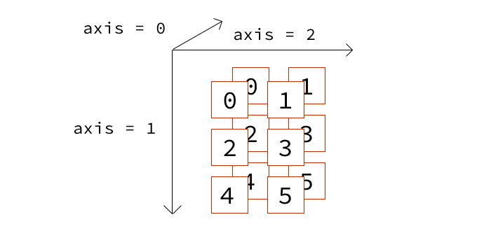
b = np.array([a, a])
b
array([[[0, 1],
[2, 3],
[4, 5]],
[[0, 1],
[2, 3],
[4, 5]]])
np.sum(b, axis=0, keepdims=True)
array([[[ 0, 2],
[ 4, 6],
[ 8, 10]]])
np.sum(b, axis=1, keepdims=True)
array([[[6, 9]],
[[6, 9]]])
np.sum(b, axis=2, keepdims=True)
array([[[1],
[5],
[9]],
[[1],
[5],
[9]]])
np.max(b, axis=0, keepdims=True)
array([[[0, 1],
[2, 3],
[4, 5]]])
np.max(b, axis=1, keepdims=True)
array([[[4, 5]],
[[4, 5]]])
np.max(b, axis=2, keepdims=True)
array([[[1],
[3],
[5]],
[[1],
[3],
[5]]])
21、多维数组乘法
对于array对象,* 和 np.multiply 函数代表的是数量积,np.dot 和 np.matmul 函数代表矩阵乘法(矢量乘法); 对于matrix对象,* 直接代表矩阵乘法(矢量乘法),np.multiply 函数表示数量积;
tensorflow乘法
1、c = tf.matmul(a, b)
二维tensor相乘 [m, k] x [k, n] = [m, n] 多维tensor相乘 [x, y, m, k] x [x, y, k, n] = [x, y, m, n],并且这里的x, y是支持广播的
2、c = tf.multiply(a, b)
按元素相乘,a, b必须形状相同,支持广播。
3、c = tf.tensordot(a, b, axes=(axes_a, axes_b))
表示任意多维,任意组合形式的矩阵相乘。(axes_a, axes_b)把 a 和 b 的元素的乘积沿着 axes_a 和 axes_b 加和。
a = tf.constant([1, 2, 3, 4])
b = tf.constant([2, 3, 4, 5])
c1 = tf.tensordot(a, b, axes=0) # axes=0则按照逐元素挨个相乘

<tf.Tensor: id=195, shape=(4, 4), dtype=int32, numpy=
array([[ 2,  3,  4,  5],
       [ 4,  6,  8, 10],
       [ 6,  9, 12, 15],
       [ 8, 12, 16, 20]], dtype=int32)>
c2 = tf.tensordot(a, b, axes=1) # 表示内积,直接令 axes=1

<tf.Tensor: id=206, shape=(), dtype=int32, numpy=40>
22、矩阵两两之间的相似性
from sklearn.metrics.pairwise import cosine_similarity
from scipy import sparse
A =  np.array([[0, 1, 0, 0, 1], [0, 0, 1, 1, 1], [1, 1, 0, 1, 0]])
A_sparse = sparse.csr_matrix(A)
similarities = cosine_similarity(A_sparse)
print('pairwise dense output:\n {}\n'.format(similarities))

#also can output sparse matrices

similarities_sparse = cosine_similarity(A_sparse, dense_output=False)
print('pairwise sparse output:\n {}\n'.format(similarities_sparse))

top_k=3
for i in range(len(similarities)):
	sim_arr = similarities[i]
	# top_index=np.argsort(sim_arr)[-top_k:]

	top_index=np.argpartition(sim_arr, -top_k)[-top_k:]
	print(str(list(zip(top_index, sim_arr[top_index]))))


# 协方差

np.cov(A)
# 相关系数

np.corrcoef(A)
23、kNN求解
import numpy as np
from numpy import ndarray

random.seed(5)

def generate_points(n: int=6) -> list[tuple]:
    points = []
    for i in range(n):
        points.append((random.randint(0, 100), random.randint(0, 100)))
    return points

def structured_array(points: list[tuple]) -> ndarray:
    dt = np.dtype([('x', 'int'), ('y', 'int')])
    return np.array(points, dtype=dt)

def np_find_dist(s_array: ndarray) -> ndarray:
    size = s_array.shape[0]
    a = s_array.reshape(size, 1)
    b = s_array.reshape(1, size)
    # 广播机制
    dist = (a['x'] - b['x'])**2 + (a['y'] - b['y'])**2
    return dist

def np_k_nearest(dist: ndarray, k: int) -> ndarray:
    k_indices = np.argpartition(dist, k+1, axis=1)[:, :k+1]
    return k_indices

def np_main(count: int = 6, top_k: int = 2):
    points = generate_points(count)
    s_array = structured_array(points)
    np_dist = np_find_dist(s_array)
    k_indices = np_k_nearest(np_dist, top_k - 1)
    # 花式索引
    results = [s_array[k_indices[i, :k+1]] for i in range(s_array.shape[0])]
    return results, s_array, k_indices, k

results, s_array, k_indices, k = np_main(100, 1)
24、稀疏举例
Coordinate (COO)
COO 格式中每一个元素用一个三元组(行号,列号,数值)表示
from scipy import sparse
rows = np.array([0, 3, 1, 0])
cols = np.array([0, 3, 1, 2])
data = np.array([6, 5, 7, 8])
sparse.coo_matrix((data, (rows, cols)), shape=(4, 4)).toarray()
array([[6, 0, 8, 0],
       [0, 7, 0, 0],
       [0, 0, 0, 0],
       [0, 0, 0, 5]])
Compressed Sparse Column (CSC)
CSC是按列存储的稀疏矩阵,其中indptr中的数据代表矩阵中每一列所存的数据在data中的开始和结束的索引,例如indptr为[0, 2, 3, 6],即表示在data中,索引[0, 2)为第一列的数据,索引[2, 3)为第二列的数据,索引[3, 6)为第三列的数据。而indices中的数据代表所对应的data中的数据在其所在列中的所在行数,例如,这里的indices为[0, 2, 2, 0, 1, 2],表示在data中,数据1在第0行,数据2在第2行,数据3在第2行,数据4在第0行,数据5在第一行,数据6在第2行。 CSC 适合做矩阵运算以及列切片,在内存中,它的元素是按列存储。
indptr = np.array([0, 2, 3, 6])
indices = np.array([0, 2, 2, 0, 1, 2])
data = np.array([1, 2, 3, 4, 5, 6])
sparse.csc_matrix((data, indices, indptr), shape=(3, 3)).toarray()
array([[1, 0, 4],
       [0, 0, 5],
       [2, 3, 6]])
Compressed Sparse Row (CSR)
CSR是按行来存储的稀疏矩阵,其与CSC类似。indptr中的数据表示矩阵中每一行的数据在data中开始和结束的索引,而indices中的数据表示所对应的在data中的数据在矩阵中其所在行的所在列数。
indptr = np.array([0, 2, 3, 6])
indices = np.array([0, 2, 2, 0, 1, 2])
data = np.array([1, 2, 3, 4, 5, 6])
sparse.csr_matrix((data, indices, indptr), shape=(3, 3)).toarray()
array([[1, 0, 2],
       [0, 0, 3],
       [4, 5, 6]])
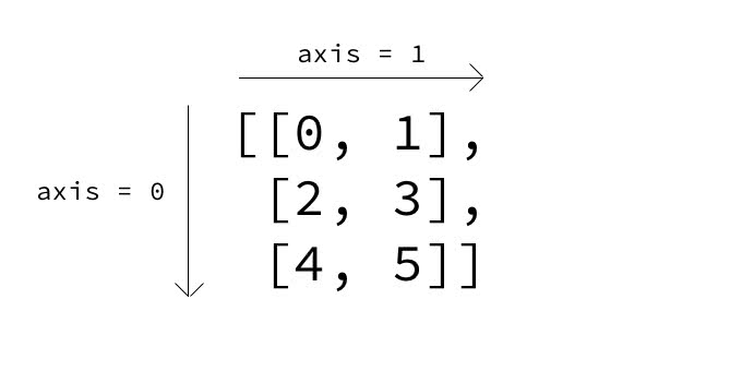
25、numpy array和tensor轴线对比
x = tf.constant([[0, 1], [2, 3], [4, 5]])
tf.reduce_sum(x)  # 15

tf.reduce_sum(x, axis=0)  # shape=(2,), array([6, 9])

tf.reduce_sum(x, axis=0, keep_dims=True)  #  shape=(1, 2) array([[6, 9]])

tf.reduce_sum(x, axis=1)  # shape=(3,) array([1, 5, 9])

tf.reduce_sum(x, axis=1, keep_dims=True)  # shape=(3, 1) array([[1],[5],[9]])

tf.reduce_sum(x, axis=-1)   # shape=(3,)  array([1, 5, 9])

tf.reduce_sum(x, axis=[0, 1])  # 15


a = np.array([[0, 1], [2, 3], [4, 5]])
np.sum(a) # 15

np.sum(a, axis=0) # array([6, 9])

np.sum(a, axis=0, keepdims=True)  # array([[6, 9]])

np.sum(a, axis=1) # array([1, 5, 9])

np.sum(a, axis=1, keepdims=True) # array([[1],[5],[9]])

np.sum(a, axis=-1) # array([1, 5, 9])
26、Numexpr优化
import numpy as np
from numpy import ndarray
import numexpr as ne

rng = np.random.default_rng(seed=4000)

def generate_ndarray(rows: int) -> np.ndarray:
    result_array = rng.random((rows, 1))
    return result_array

arr = generate_ndarray(10)


def numexpr_to_binary(np_array: np.ndarray) -> np.ndarray:
    # N * 1 -> N
    temp = np_array[:, 0]
    temp = ne.evaluate("where(temp<0.5, 0, 1)")
    # N -> N * 1
    return temp[:, np.newaxis]

arr = generate_ndarray(10)
result = numexpr_to_binary(arr)

mapping = np.column_stack((arr, result))
mapping